
Today AI assistants are taking more and more place in our life and most of us have already used one in the past few months. But how are they working? How can they learn? It’s a fascinating question and we’ll need more than an article to explain it. However, we can start by thinking about the “base” of this technology, neural networks, used to learn how to compute an input to give a result as close as the attempted one.
It uses “deep learning concept” in “machine learning”. To do so I will guide you with an example in GO running in a Google Colab environment. Why go? Because when we talk about AI, most of the time you have code in python but we hardly use GO at Bedrock. Why Google Colab? Because it’s an easy way to have the same, shareable, environment.
📚 Concepts
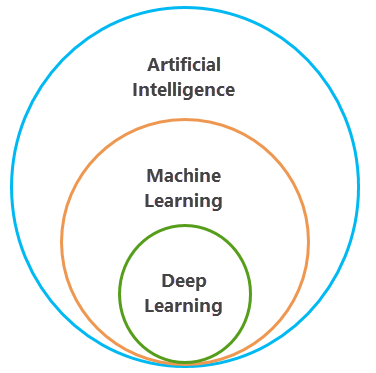
Deep learning
Deep learning is a part of the AI family.
I will not give a detailed definition about IA or machine learning, because it’s not the purpose of this article. I will just give some definitions about AI and machine learning to help understanding what lies behind these terms.
AI “The construction of computer programs that engage in tasks which, for now, are performed more successfully by human beings, as they require high-level mental processes such as perceptual learning, memory organization, and critical reasoning.” AI is not limited to LLM and other Data generation or classification. For example, an algorithm capable of finding the fastest path to a destination can fit the definition without modern concepts. Machine learning Allows a machine to ‘learn’ to solve a problem based on a model by minimizing the errors between the model’s results and our data through an optimization algorithm. It can be a neural network or just a function. Deep learning It’s a way to apply machine learning on complex systems (neural network, will see it in the next chapter) by using methods to calculate and fix error layer by layer (you may have heard about “back propagation”, “gradient”, etc.).
As you can see, what we recently call “AI” (LLM and image generation) are a small part of AI. Their common point is learning by minimizing an error which looks like the way humans learn but in fact it’s slightly different. Modern AI are using different “systems” to encode input and learn how to find the right solution. This post will focus on the base of the system : how it computes an output from an input?
Let’s take an example :
Imagine you have a sample of data with 2 values : X and Y which can be the width and the height of a leaf from a tree and you want to know if its fruits are edible. You record a sample of data and order them by edible (green) or not (yellow).
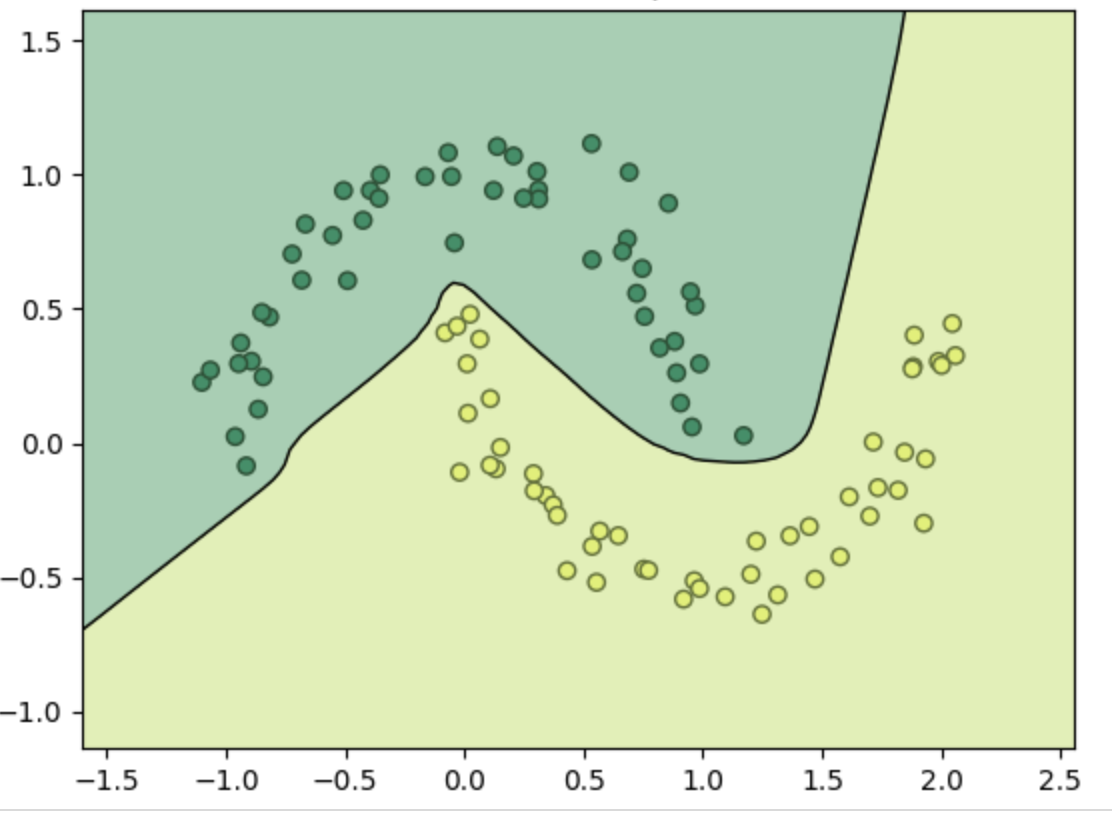 As you can see we can delimit a frontier where edible and inedible are separated.
Of course it’s a “simple” example but the goal of deep learning is to find a way to configure the system so it can find a kind of frontier and predict a result (in our example if it’s edible or not).
When an AI learns how to find a way to “predict” if the fruit is edible from its leaf, it tries to find a formula which will do minimal errors.
As you can see we can delimit a frontier where edible and inedible are separated.
Of course it’s a “simple” example but the goal of deep learning is to find a way to configure the system so it can find a kind of frontier and predict a result (in our example if it’s edible or not).
When an AI learns how to find a way to “predict” if the fruit is edible from its leaf, it tries to find a formula which will do minimal errors.
Neuron based system
Since the beginning we are talking about a “system” which can learn. What we call “system” is a number of little compute units called “neurons”. Each one makes a simple computation but by connecting them to each other in several layers we can do complex things.
First let’s talk about neurons. A neuron is inspired by biological neurons :
- biological neurons send a signal depending on their inputs (dendrites). They make an addition about received signals and “decide” if they should activate their output (axon). The decision uses complex biological concepts but we can simplify it by saying it gives different attention to the given inputs, and decides if it should produce a signal (output).
- logical neurons do the same, they compute their inputs (X1 … xn), decide with a function to give different attention depending on the inputs and if they should activate (send a value > 0) and send an output or not.
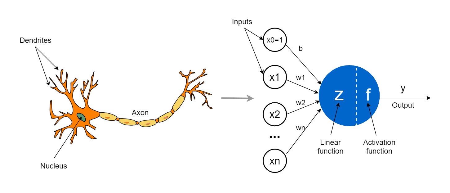
We will not go into more detail about how it works or how to classify data (like in the example above with the dots). Just remember that a neural network unit (a neuron) applies a function to its inputs using several parameters to increase or decrease the influence (or weight) of each input. It then applies an activation function to the result to produce the final output. So, a neuron is defined with 2 functions:
- The one which increase/decrease inputs
- The one which take all the increased/decrease inputs and choose if it should produce a result
The first one is a simple equation : X1W1 + X2W2 + b where X1, X2 are the inputs, and W1-W2 the “weight” of each input which can increase or decrease their value. This example is for 2 inputs but you can have as many as you want inputs. Each input should have a weight and will be added to the others.
There is only one “b” which is the bias of the neuron. The bias prevents the neuron’s decision boundary line from always going through the origin (0,0). In this case the network would become less flexible.
The second one is chosen depending on the input we want and the goals of a neural network. Because we are using a single neuron, let’s say this function does nothing and returns the result of the equation.
Finally, we have a neuron which is a function X1W1 + X2W2 + b which will return the result of the equation as an output.
How can we make it learn?
⚙ Let’s experiment
Sometimes an example is better than a long sentence. Let’s create a neuron in GO on Google Colab. We’ll give it 2 integers as an input (i.e. 1 and 2) and we tell it it has to find 5 as an output.
So the equation will look like 1W1 + 2W2 + b = 5 .
Of course there is several easy ways to resolve it and maybe you will use mathematics to find these solutions.
But don’t forget our neuron is “naïve”, it does not know anything about maths or equations. It will just learn with the fail/retry method.
How a neuron “learn”
It would be too long to explain it deeply. You just have to know the workflow of compute/test/correct/retry :
- start with random parameters w1/w2 and B
- take inputs given by the user
- compute the result and compare it with the attempted one, which we call the error
- change the params to come closer to the attempted result
- restart @1
The tricky parts are part 3 and 4: How a neuron could find how far from the attempted result it is and how much it should update the params to reduce the loss?
The Loss function
First you need to know how the neuron will evolve its output depending on the params.
The loss function does something like this : it measures the “level of error” of your model comparing predicted vs attempted value. The less the result of the function is, the more accurate your model is.
For example if you have 5 as attempted value but the model find 3, the loss could be the % of accuracy is 3*100/5=60%, so the error could be 40%
One of popular loss function is the log loss function :
So you want to find a way to go to the lowest point which should be where you have a model with the best predictions (= with few errors).
Gradient
Now we know how to calculate the “error level” of our model, how should we vary its params to get closer to the best values with a minimal loss value? We use a method called “gradient”: In mathematics, the gradient is a way to describe how a function changes — it tells you the direction and rate of the steepest increase of that function. The gradient is the vector of partial derivatives of the loss function with respect to its parameters. Don’t panic, just remember it’s a kind of derivative which tells us if the error is decreasing or increasing and how fast. The gradient use the loss function to find out for each param the equation which describe how, if we increase or decrease this param, the error change (better/worst) For example if it returns -2 it means you are decreasing the error with a “speed” of 2. So you want to update your params by decreasing them by 2 (remember it’s a very simplified explanation, you can learn more on AI courses).
🧪 Experiment
Ready? Let’s experiment it!
We will create a neuron which will learn how to find the solution of this equation : x1w1 + x2w2 + b = y
We will give him x1, x2 and the wanted result y.
=> The neuron will learn, without any mathematical knowledge, how to find the result y with given x1 and x2
Environment configuration
First you will need to configure your environment We are going to use Google Colab tool because it’s easy to configure, you can work with multiple people on it, it’s automatically versionned and saved and it’s easy to share. First you have to upload this jupyter file notebook :
- Go to colab
- Click on
Uploadand chose the jupyter notebook
Concept and code explanation
The notebook first initialize the environment to be able to launch go and compute the code. It also use python to display results (more comfortable as it’s natively supported by Google Colab).
!wget https://go.dev/dl/go1.21.1.linux-amd64.tar.gz
!sudo rm -rf /usr/local/go
!sudo tar -C /usr/local -xzf go1.21.1.linux-amd64.tar.gz
!export PATH=$PATH:/usr/local/go/bin
import os
os.environ["PATH"] += ":/usr/local/go/bin"
Then you have the neuron.go file which describe the neuron model.
%%writefile neurone.go
package main
...
You will find in this file:
Initialization function func initialisation() ([2]float64, float64)
=> will initialize neuron params (W1 and W2 in array W := [2]float64{normal(), normal()} and bias b) with random value (these values will be updated during training by the model)
The model, which is the function which calculates an output z by applying weights on inputs
z := X[0]*W[0] + X[1]*W[1] + b
The loss function, used to know how far from the attempted result we are
func loss(a, y float64) float64 {
	return (y - a)
}
The gradient (gap function) which will return new weights, adjusted from the error
func gap(a float64, X [2]float64, y float64) ([2]float64, float64)
The update function, which will update current params (weight and bias) , proportionally from a step value, with the fix returned by the gradient.
func update(dW [2]float64, db float64, W [2]float64, b float64, learningRate float64) ([2]float64, float64)
These functions are used in our neuron model to learn and find the solution with right w1, w2 and b values
func artificialNeuron(X [2]float64, y float64, learningRate float64, nIter int) ([2]float64, float64)
Finally you have exportData which will export learning data to display the learning curve with python (because it’s easier :D ) and the main function to launch the learning process and display learning results.
Please note the given inputs X1 = 1.0, X2 = 2.0 and attempted output Y = 5
X := [2]float64{1.0, 2.0}
y := 5.0
Let’s learn !
Launch each part of the jupyter by clicking on the black play icon :
![]()
Results
for each runned part, you will get an output.
for neurone.go file you’ll have a message to confirm the file creation (or overwrite if you already loaded it)
Overwriting neurone.go
Then after launching the execution of the main go file neurone.go you’ll receive this stack :
Initial W: [-0.7639828855477203 -0.23618327598412134] b: 1.242355565991255

iteration 1-------------------------
Current X: [1 2]
Current W: [-0.7639828855477203 -0.23618327598412134] b: 1.242355565991255
accuracy 0.12012256950584277
Updated W: [-0.2645834983952495 0.7626154983208203] b: 1.741754953143726

iteration 2-------------------------
Current X: [1 2]
Current W: [-0.2645834983952495 0.7626154983208203] b: 1.741754953143726
accuracy 60.04804902780235
Updated W: [-0.06482374353426118 1.1621350080427968] b: 1.9415147080047142

iteration 3-------------------------
Current X: [1 2]
Current W: [-0.06482374353426118 1.1621350080427968] b: 1.9415147080047142
accuracy 84.01921961112092
Updated W: [0.015080158410134187 1.3219428119315875] b: 2.0214186099491096

iteration 4-------------------------
Current X: [1 2]
Current W: [0.015080158410134187 1.3219428119315875] b: 2.0214186099491096
accuracy 93.60768784444836
Updated W: [0.04704171918789237 1.3858659334871037] b: 2.053380170726868

iteration 5-------------------------
Current X: [1 2]
Current W: [0.04704171918789237 1.3858659334871037] b: 2.053380170726868
accuracy 97.44307513777936
Updated W: [0.059826343498995536 1.41143518210931] b: 2.066164795037971

iteration 6-------------------------
Current X: [1 2]
Current W: [0.059826343498995536 1.41143518210931] b: 2.066164795037971
accuracy 98.97723005511175
Updated W: [0.0649401932234368 1.4216628815581926] b: 2.0712786447624123

iteration 7-------------------------
Current X: [1 2]
Current W: [0.0649401932234368 1.4216628815581926] b: 2.0712786447624123
accuracy 99.5908920220447
Updated W: [0.06698573311321336 1.4257539613377457] b: 2.073324184652189

iteration 8-------------------------
Current X: [1 2]
Current W: [0.06698573311321336 1.4257539613377457] b: 2.073324184652189
accuracy 99.83635680881788
Updated W: [0.06780394906912397 1.4273903932495668] b: 2.0741424006080997

iteration 9-------------------------
Current X: [1 2]
Current W: [0.06780394906912397 1.4273903932495668] b: 2.0741424006080997
accuracy 99.93454272352714
Updated W: [0.06813123545148825 1.4280449660142953] b: 2.074469686990464

iteration 10-------------------------
Current X: [1 2]
Current W: [0.06813123545148825 1.4280449660142953] b: 2.074469686990464
accuracy 99.97381708941086
Updated W: [0.06826215000443395 1.4283067951201867] b: 2.07460060154341


End-------------------
Final weights (params) : [0.06826215000443395 1.4283067951201867] Final bias : 2.07460060154341
Prediction : 4.999476341788217
you can see the inital weights (params) and bias.
Initial W: [-0.7639828855477203 -0.23618327598412134] b: 1.242355565991255
the original accuracy in percent : accuracy 0.12012256950584277 .
Then the neuron start learning and the accuracy increase to reach 99.97% You can see weights and bias changing during the learning phase
For each iteration you can see
- iteration name :
iteration 1------------------------- - input received (train data) :
Current X: [1 2] - current weights :
Current W: [-0.7639828855477203 -0.23618327598412134] b: 1.242355565991255 - current accuracy:
accuracy 0.12012256950584277 - Update weights (after the model calculate the adjustements):
Updated W: [-0.2645834983952495 0.7626154983208203] b: 1.741754953143726
The last 2 lines give you final results:
- params
W1=-0.07,w2=1.43and bias b=2.07. - prediction : the output result
4.999(reminder: we attempted 5 it’s very very close)
If you try it: 10.06826215000443395 + 21.4283067951201867 + 2.07460060154341 and you get 4,999476341788217 🎉
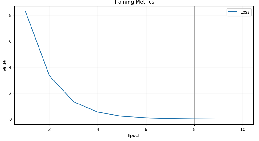
You can also see the “loss” decreasing during the learning phase : The more the neuron learn the less the value of the loss is and the more the accuracy is !
👨🏻🏫 Conclusions
As you can see, a neuron can learn without any knowledge, just by giving it data and applying mathematical concepts to make it “learn”. If you launch multiple times the learning process, you may find a different result (because initial values may vary). In fact, this example is useless in the real world because we can resolve the problem by ourselves. This is why “neural networks”, used in most AI like text generation, image detection or generation, are using thousand of neuron! But now you know the “basic concepts” and maybe understand more how an AI agent learns!